Supervised Learning : classification

Supervised learning is the branch of Machine Learning (ML) that involves predicting labels, such as ‘Survived’ or ‘Not’. Such models learn from labelled data, which is data that includes whether a passenger survived (called “model training”), and then predict on unlabeled data.

These are generally called train and test sets because

You want to build a model that learns patterns in the training set, and
You then use the model to make predictions on the test set.

We can then calculate the percentage that you got correct: this is known as the accuracy of your model.

2.1. Leakage

2.2. Metrics

2.3. hyper-parameter optimization

the catalogue

3.1 Random Forests

3.2 Naive Bayes

3.3 SVM

back to ToC

How To Start with Supervised Learning

As you might already know, a good way to approach supervised learning is the following:

Perform an Exploratory Data Analysis (EDA) on your data set;
Build a quick and dirty model, or a baseline model, which can serve as a comparison against later models that you will build;
Iterate this process. You will do more EDA and build another model;
Engineer features: take the features that you already have and combine them or extract more information from them to eventually come to the last point, which is
Get a model that performs better.

A common practice in all supervised learning is the construction and use of the train- and test- datasets. This process takes all of the input randomly splits into the two datasets (training and test); the ratio of the split is usually up to the researcher, and can be anything: 80/20, 70/30, 60/40…

There are various classifiers available:

Decision Trees – These are organized in the form of sets of questions and answers in the tree structure.
Naive Bayes Classifiers – A probabilistic machine learning model that is used for classification.
K-NN Classifiers – Based on the similarity measures like distance, it classifies new cases.
Support Vector Machines – It is a non-probabilistic binary linear classifier that builds a model to classify a case into one of the two categories.
…

We will mostly focus on decisions trees for now, to explore and experiment core concepts of the classification pipeline in Machine Learning.

Once these concepts are well understood, it is actually relatively easy to apply them to more and more algorithms.

back to ToC

1. our first classifier : Decision trees

It is a type of supervised learning algorithm. We use it for classification problems. It works for both types of input and output variables. In this technique, we split the population into two or more homogeneous sets. Moreover, it is based on the most significant splitter/differentiator in input variables.

The Decision Tree is a powerful non-linear classifier. A Decision Tree makes use of a tree-like structure to generate relationship among the various features and potential outcomes. It makes use of branching decisions as its core structure.

There are two types of decision trees:

Categorical (classification) Variable Decision Tree: Decision Tree which has a categorical target variable.
Continuous (Regression) Variable Decision Tree: Decision Tree has a continuous target variable.

Regression trees are used when the dependent variable is continuous while classification trees are used when the dependent variable is categorical. In continuous, a value obtained is a mean response of observation. In classification, a value obtained by a terminal node is a mode of observations.

The main advantages of the decision tree is :

no need to scale your data
ability to do non-linear classification
resulting models are easy to interpret

Here, we will use the rpart and the rpart.plot package in order to produce and visualize a decision tree. First of all, we’ll create the train and test datasets using a 70/30 ratio and a fixed seed so that we can reproduce the results.

# split into training and test subsets
library(caret)
set.seed(1000)
inTraining <- createDataPartition(breastCancerData$Diagnosis, p = .70, list = FALSE)
breastCancerData.train <- breastCancerDataNoID[ inTraining,]
breastCancerData.test  <- breastCancerDataNoID[-inTraining,]

Now, we will load the library and create our model. We would like to create a model that predicts the Diagnosis based on the mean of the radius and the area, as well as the SE of the texture. For ths reason we’ll use the notation of myFormula <- Diagnosis ~ Radius.Mean + Area.Mean + Texture.SE. If we wanted to create a prediction model based on all variables, we will have used myFormula <- Diagnosis ~ . instead.

The decision tree algorithm comes with a number of parameters which reflect the following aspects of the model:

minsplit: the minimum number of instances in a node so that it is split
minbucket: the minimum allowed number of instances in each leaf of the tree
maxdepth: the maximum depth of the tree
cp: parameter that controls the complexity for a split and is set intuitively (the larger its value, the more probable to apply pruning to the tree)

These parameters of the methods which are not set directly from our data itself are called hyper-parameters.

library(rpart)
library(rpart.plot)
myFormula <- Diagnosis ~ Radius.Mean + Area.Mean + Texture.SE

breastCancerData.model <- rpart(myFormula,
                                method = "class",
                                data = breastCancerData.train,
                                minsplit = 10,
                                minbucket = 1,
                                maxdepth = 3,
                                cp = -1)

print(breastCancerData.model$cptable)
rpart.plot(breastCancerData.model)

We see the following output and a figure:

Full decision tree

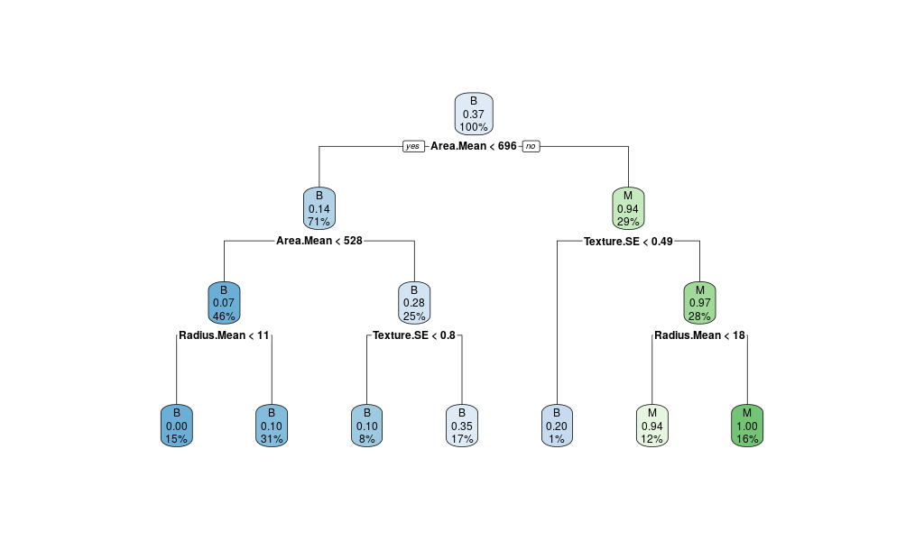
           CP nsplit rel error    xerror       xstd
0.69127517      0 1.0000000 1.0000000 0.06484708
0.02013423      1 0.3087248 0.3087248 0.04281476
0.00000000      2 0.2885906 0.3154362 0.04321630
-1.00000000      6 0.2885906 0.3154362 0.04321630

Here, you can see that different values of CP have been explored. Interestingly, each value tested are associated with :

rel error : relative error
xerror : cross-validation error (rpart does a 10-fold cross validation without telling you, how nice!)

As we can observe, the value with the lowest relative error (CP: -1), does not correspond to the value with the lowest cross-validation error (CP:0.2013423)

Question: Why is that? Which one should we try to optimize?

Let’s select the tree with the minimum prediction error:

errorType = "xerror" # would you choose "rel error" or "xerror" ?
opt <- which.min(breastCancerData.model$cptable[, errorType])
cp <- breastCancerData.model$cptable[opt, "CP"]
# prune tree
breastCancerData.pruned.model <- prune(breastCancerData.model, cp = cp)
# plot tree
rpart.plot(breastCancerData.pruned.model)

table(predict(breastCancerData.pruned.model, type="class"), breastCancerData.train$Diagnosis)

The output now is the following Confusion Matrix and pruned tree:

    B    M
B  245  34
M   9   109

Pruned decision tree

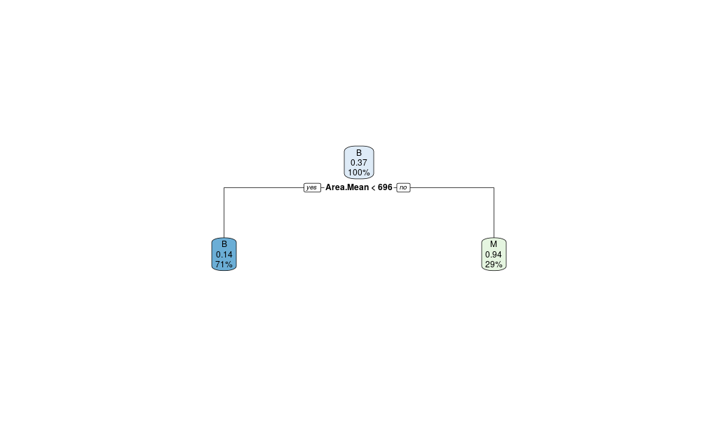
Question: What does the above “Confusion Matrix” tells you?

So when it increases the CP parameter’s effect will reduce the performance on the train set (rel error), but limit the amount of error done on new data (xerror). In other words, it can help avoid overfitting of the model. In a sense it is a regularization parameter.

Regularization is a double edged sword:

too little regularization : overfitting on the train set, bad performance on new data (eg. test set)
too much regularization : bad performance overall

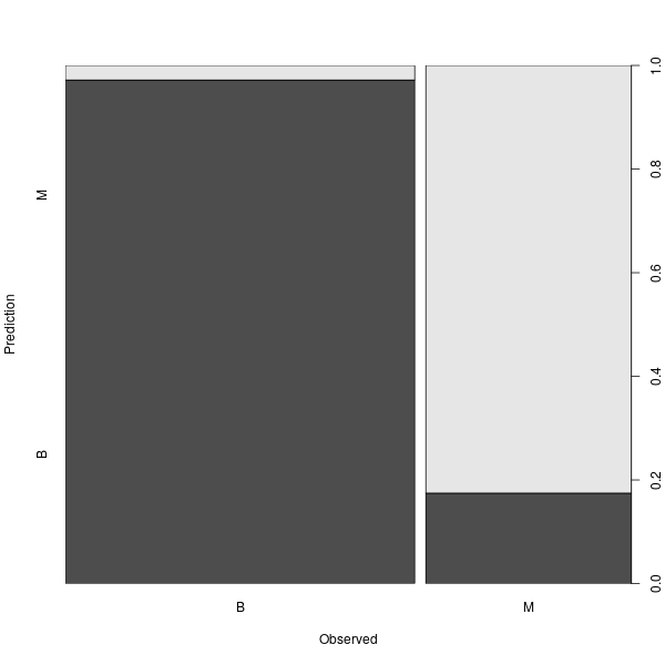
Anyway, now that we have a model, we should check how the prediction works in our test dataset.

## make prediction
BreastCancer_pred <- predict(breastCancerData.pruned.model, newdata = breastCancerData.test, type="class")
plot(BreastCancer_pred ~ Diagnosis, data = breastCancerData.test,
     xlab = "Observed",
     ylab = "Prediction")
table(BreastCancer_pred, breastCancerData.test$Diagnosis)

The new Confusion Matrix is the following:

BreastCancer_pred   B   M
                B 104  11
                M   3  52

Prediction Plot

Exercises
1	Can we improve the above model? What are the key hyperparameters that have the most impact?
2	We have been using only some of the variables in our model. What is the impact of using all variables / features for our prediction? Is this a good or a bad plan?

back to ToC

2. “The classiciation pipeline”

Now that we have experimented a little with a type model (decision tree), we will be able to discuss important aspects of classification routines in Machine Learning: what are the aspects that are common to most approaches ? what to strive for ? which pitfall to avoid ?

2.1. Leakage - the insidious foe

Consider the following code, which explores different values for the parameter maxdepth:

v.maxdepth = 1:10
v.xerror = c()
v.predError = c()

for(maxdepth in v.maxdepth){

  breastCancerData.model <- rpart( 'Diagnosis ~ . ' ,
                                method = "class",
                                data = breastCancerData.train,
                                minsplit = 10,
                                minbucket = 1,
                                maxdepth = maxdepth,
                                cp = -1)


  opt <- which.min(breastCancerData.model$cptable[, "xerror"])

  cp <- breastCancerData.model$cptable[opt, "CP"]
  breastCancerData.pruned.model <- prune(breastCancerData.model, cp = cp)


  xerror = min( breastCancerData.model$cptable[, "xerror"] )
  predError = mean( predict(breastCancerData.pruned.model, newdata = breastCancerData.test, type="class") != breastCancerData.test$Diagnosis )

  v.xerror = c(v.xerror , xerror)
  v.predError = c(v.predError , predError)
}


plot(v.maxdepth , v.xerror , type='l' , lwd=2, 
	ylim=c(0.0,1.0) , xlab='maxdepth' , ylab='error')
lines(v.maxdepth , v.predError  , col='red', lwd=2)

legend('topright', c('cross-validation error' , 'prediction error') , lwd=2, col=c('black','red'))

m = which.min(v.xerror)
points(v.maxdepth[m] , v.xerror[m]  , col='black', lwd=2)
m = which.min(v.predError)
points(v.maxdepth[m] , v.predError[m]  , col='red', lwd=2)

maxdepth exploration

Where the little circle mark the points where a minimum is reached.

Question:Which maxdepth should I choose here for my final model?

back to ToC

2.2. Metrics

So far, we searching for the best possible model we have been fairly elusive about what “best” actually means. Intuitively, we mean we would like a model that makes as little “error” as possible. In practice, this comes down to optimizing a metric.

There are several metrics which differ in the importance they give to different types of errors (False Positive, False Negative), or how they handle different kinds biases, in particular imbalance.

Confusion Matrix	Predicted NO	Predicted YES
Actual NO	TN	FP
Actual YES	FN	TP

Note : these rely on the definition of one category as the TRUE one, and the other as the FALSE one. For some measures this choice is not without consequences

Aparte : imbalance

Imbalance describes the idea that in your (training) data one of the class is over-represented with respect to the other.

Consider for instance a situation where the training data is made of 990 observations of category NO, and 10 of category YES. Now, imagine we create a classifier for this model which will be evaluated on a metric called Accuracy, which is the default metric in most implementations:

Accuracy = (TP + TN)/ N

, where N is the total number of observations.

From there, even a “uninteresting” classifier which just, without even looking at the data, classifies everything as NO would get a good performance:

Uninteresting Classifier	Predicted NO	Predicted YES
Actual NO	990	0
Actual YES	10	0

Acc_uninteresting = 990/(990+10) = 0.99

Back on track

Here is a non exhautive list of common metrics you can use :

Name	formula	sensitive to imbalance	`caret`
Sensitivity , Recall	TP/(TP+FN)	YES	`'Sens'`
Specificity	TN/(FP+TN)	YES	`'Spec'`
Precision	TP/(TP+FP)	YES	`'Precision'`
Accuracy	(TP + TN)/ N	YES	`'Accuracy'`
F1-measure	2 * (precision * recall)/(precision + recall)	YES	`'F'`
ROC AUC	area under the ROC curve	NO	`'ROC'`
Cohen’s Kappa	2 * (TPTN - FNFP)/((TP+FP)(FP+TN)+(TP+FN)(FN+TN))	LESS	`'Kappa'`

ROC AUC example

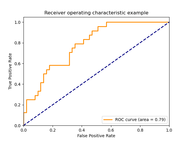
Additionnaly, you can see that this only covers cases where there is only 2 classes (binary case), other metrics exists or have been adapted for multi-class problems.

back to ToC

2.3. hyper-parameter optimization

So our goal is to find the best set of hyperparameters for our classification model.

We have already seen that using a form of cross-validation method is key to avoid both overfitting and leakage.

So far, what we have done is to explore combinations of a fixed number of parameter values in a systematic manner : the grid search While crude, this method is actually quite valid.

Alternatives exist, such as drawing parameter values to test randomly, or using a bayesian-based algorithm for instance.

For the frame of this course, the grid search is more than enough.

When it comes to parameter tuneing, the interface of the caret library can be somewhat lacking. Plainly said, it can only tune a small fraction of available hyperparameters for each algorithm, so we have to code a solution around the library (which can sometimes be tedious).

Indeed, consider the single decision tree:

# getModelInfo returns the hyperparameters which are tunable using caret train function
getModelInfo( 'rpart' , regex=FALSE)[[1]]$parameters

  parameter   class                label
1        cp numeric Complexity Parameter

Only cp is tuned directly, out of the 4 main hyperparameters (minsplit, minbucket, maxdepth, cp)…

This is not a coding course per se, so here is a simplistic function which should provide a simple interface for most of your experimentations during this workshop.

Let’s still take the time to dissect it a little: this should give you interesting insight on how caret works and how you could later on look at alternative aspects of the algorithm (eg. change from K-fold cross validation to leave-one-out validation, use your own metrics, add preprocessing into the mix, …)

# to facilitate hyperparameter tuning and playing around with different metrics, I have implemented my own grid search function built around caret::train
GridSearchCV = function( F ,data , mName,paramSpace,K=10 ,metric="Accuracy" )
{
    
    obligate = getModelInfo( mName , regex=FALSE)[[ mName ]]$parameters$parameter
    
    non_obligate = names(paramSpace)[ ! names(paramSpace) %in% obligate ]
    
    non_obligateGrid <- do.call( expand.grid , paramSpace[ non_obligate ] )
    obligateGrid <- do.call( expand.grid , paramSpace[ obligate ] )

    sumFun = defaultSummary
    classProbs = FALSE
    if( metric %in% c('ROC','Sens','Spec') ){
    	sumFun = twoClassSummary
    	classProbs = TRUE
    }
    if( metric %in% c('Precision','Recall','F','AUC') ){
    	sumFun = prSummary
    	classProbs = TRUE
    }
    
    fitControl <- trainControl(## K-fold CV
                               method = "cv",
                               number = K,
                               classProbs = classProbs , summaryFunction =  sumFun) 
    
    result = data.frame()
    
    for( i in 1:nrow(non_obligateGrid) ){
    
    argList1 = as.list( non_obligateGrid[i,] )
    names(argList1) = colnames(non_obligateGrid)
    
    print(paste("testing", non_obligateGrid[i,] ))
    
    argList2 = list( form = F , data = data , method = mName , trControl = fitControl , metric = metric , maximize=TRUE, tuneGrid= obligateGrid )
    
    argList = c(argList2,argList1)
    
    rfFit <- do.call(caret::train , argList)
    
    resTmp = cbind(non_obligateGrid[i,],rfFit$results[,c(obligate , metric)])
    names( resTmp ) = c( non_obligate , obligate , metric )
    
    result = rbind( result , resTmp )
    }
    
    
    return( result )
}

#example usage
GridSearchCV( F = Diagnosis ~ .,data = breastCancerData.train,
            mName = 'rpart',
            paramSpace = list( cp=c(-1,0,0.1,0.3) , maxdepth = seq(2,8,2)  ) , metric='Accuracy' )

   maxdepth   cp  Accuracy
       2 -1.0 0.9323718
       2  0.0 0.9348718
       2  0.1 0.8922436
       2  0.3 0.8922436
       4 -1.0 0.9399359
       4  0.0 0.9399359
       4  0.1 0.8998077
       4  0.3 0.8998077
       6 -1.0 0.9349359
      6  0.0 0.9349359
      6  0.1 0.8997436
      6  0.3 0.8997436
      8 -1.0 0.9248718
      8  0.0 0.9248718
      8  0.1 0.8999359
      8  0.3 0.8999359

From there, you can train a model with the best hyper-parameter found.

If you are intersted, you can have a read at this article which proposes (toward the end) a somewhat more elegant (if less generalistic) alternative to extend caret functionnalities.

Exercise : Your turn to play! Tune a decision tree hyper-parameters.

choose appropriate hyper-parameter ranges to test (Warning : grid search can take a while to run if you are too extensive)
test different metrics. What is an appropriate metric here ? is there imbalance ? what is our goal in this classification ?

Take you time. Experiment. Have fun.

back to ToC

3. the catalogue

From there, you have most of the core tools and concepts you need to deploy a simple Machine Learning classification task.

The next step is to accumulate a “catalogue” of different algorithms you will feed you pipeline instead of the “single decision tree” we have been using until now.

We will review here a few of the most common algorithms.

You can alway consult the extensive list of available models in caret for more.

3.1 Random Forests

Random Forests is an ensemble learning technique, which essentially constructs multiple decision trees. Each tree is trained with a random sample of the training dataset and on a randomly chosen subspace. The final prediction result is derived from the predictions of all individual trees, with mean (for regression) or majority voting (for classification). The advantage is that it has better performance and is less likely to overfit than a single decision tree; however it has lower interpretability.

There are two main libraries in R that provide the functionality for Random Forest creation; the randomForest and the party: cforest().

Package randomForest

very fast
cannot handle data with missing values
a limit of 32 to the maximum number of levels of each categorical attribute
extensions: extendedForest, gradientForest

Package party: cforest()

not limited to the above maximum levels
slow
needs more memory

In this exercise, we will be using the randomForest, which is somewhat the default random forest algorithm in caret (model name 'rf').

First, let’s train a model:

library(randomForest)
set.seed(1000)
rf <- randomForest(Diagnosis ~ ., data = breastCancerData.train,
                   ntree=1000,
                   proximity=T)

table(predict(rf), breastCancerData.train$Diagnosis)

The output is the following:

   B   M
B 245   9
M   5 139

We can also investigate the content of the model:

print(rf)

The output shows the individual components and internal parameters of the Random Forest model.

Call:
 randomForest(formula = Diagnosis ~ ., data = breastCancerData.train,      ntree = 1000, proximity = T) 
               Type of random forest: classification
                     Number of trees: 1000
No. of variables tried at each split: 5

        OOB estimate of  error rate: 3.51%
Confusion matrix:
    B   M class.error
B 245   5  0.02000000
M   9 140  0.06040268

Note the number of variables tried at each split : 5, this is an important hyper-parameter.

We can view the overall performance of the model here:

plot(rf, main = "")

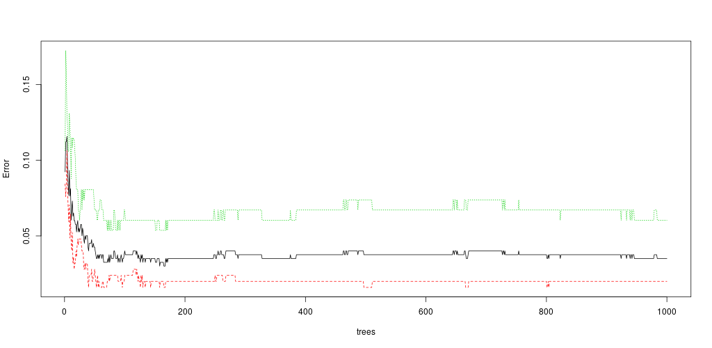
Error rate plot for the Random Forest model

As you can see, the number of trees can (sometimes) act as an regularization parameter:

too few tree: underfitting
too much tree: overfitting

We can also review which of the variables has the highest “importance” (i.e. impact to the performance of the model):

importance(rf)

varImpPlot(rf)

The output is the table and the figure below:

                        MeanDecreaseGini
Radius.Mean                    7.0287698
Texture.Mean                   2.6388944
Perimeter.Mean                 7.4826035
Area.Mean                      9.3068041
Smoothness.Mean                1.1433273
Compactness.Mean               2.8390791
Concavity.Mean                10.0168335
Concave.Points.Mean           20.8914978
Symmetry.Mean                  1.0771518
Fractal.Dimension.Mean         0.7794169
Radius.SE                      2.2249672
Texture.SE                     0.9978639
Perimeter.SE                   2.4517692
Area.SE                        5.4191539
Smoothness.SE                  0.7963913
Compactness.SE                 0.7643879
Concavity.SE                   1.5406829
Concave.Points.SE              0.9562777
Symmetry.SE                    0.9148704
Fractal.Dimension.SE           0.9435165
Radius.Worst                  18.3375362
Texture.Worst                  3.7577203
Perimeter.Worst               22.2321797
Area.Worst                    21.1024195
Smoothness.Worst               2.6922458
Compactness.Worst              3.7267283
Concavity.Worst                6.6297564
Concave.Points.Worst          24.0075265
Symmetry.Worst                 2.0081243
Fractal.Dimension.Worst        1.8349326

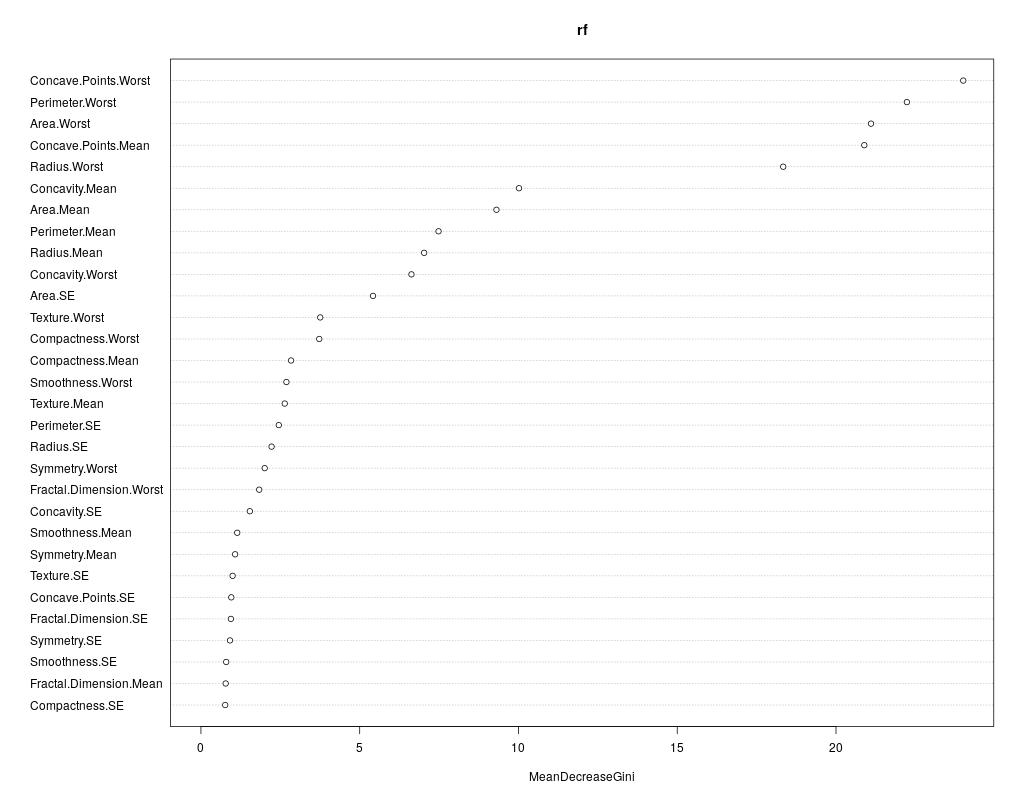
Importance of the individual variables

Question: What could that be useful for?

Let’s try to do a prediction of the Diagnosis for the test set, using the new model. The margin of a data point is as the proportion of votes for the correct class minus maximum proportion of votes for other classes. Positive margin means correct classification.

BreastCancer_pred_RD <- predict(rf, newdata = breastCancerData.test)
table(BreastCancer_pred_RD, breastCancerData.test$Diagnosis)

plot(margin(rf, breastCancerData.test$Diagnosis))

The output is the table and figure below:

BreastCancer_pred_RD   B   M
                   B 105   4
                   M   2  59

Margin plot for the Random Forest

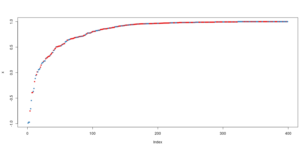
The margin of a data point is defined as the proportion of votes for the correct class minus maximum proportion of votes for the other classes. Thus under majority votes, positive margin means correct classification, and vice versa.

So now, what is left is how to integrate this into our grid-search to find optimal hyperparameters.

The name of the model is 'rf' in caret. A look at the help : ?randomForest will show you a lot of potentially interesting hyperprarameters. The most important are:

mtry: Number of variables randomly sampled as candidates at each split (obligatory for caret train)
ntree : Number of trees to grow.

Exercise : Your turn to play! Tune a random hyper-parameters, train a model and try to draw conclusions from it.

We mentionned 2 main hyper-parameters: mtry and ntree. Do you see others you would like to test?
Between you best random forest and your best single decision tree classifier, which one would you prefer? why?

back to ToC

3.2 Naive Bayes

library(klaR)
?NaiveBayes

caret method name : nb.

Important hyper-parameters:

usekernel : if TRUE a kernel density estimate (density) is used for density estimation. If FALSE a normal density is estimated.
fL : Factor for Laplace correction, default factor is 0, i.e. no correction. The higher it is, the more regulization. article on this correction. A typical range could be between 0 and 1.
adjust : the bandwidth used is actually adjust*bw. This makes it easy to specify values like ‘half the default’ bandwidth.

Exercise : you know the drill by now, so your turn to play!

back to ToC

3.3 SVM

library(kernlab)

SVM comes in different flavors, depending on the type of kernel used to combine features.

linear kernel, 'svmLinear' : the mapping of observations use a linear composition of variables.

C : “cost” : tells the SVM optimization how much you want to avoid misclassifying each training example. This is an inverse-regularization parameter (higher = less regularization). Typical range is 1e-6 to 10 (use a log-scale). The second answer to this stack overflow post gives a nice visual example.

polynomial kernel, 'svmPoly' : now we use a polynomial combination of features

C : same as before
degree : degree of the polynome to use (integer values)
scale : a factor applied on variables which is sometimes used to normalize patterns(?). typycally between 1e-3 and 1 (use log-scale)

radial basis function kernel (RBF) 'svmRadial', uses a form of euclidian distance around each point.

C : same as before
sigma : scaling on how the “influence” of a point diminishes with distance. Regularizing hyperparameter. Also often seen as gamma = 1/2*sigma^2. Typical range between 0.01 and 1000.

There is not much to say and you could just go to practise with this new algorithm like before. Except there is an interesting twist: SVM requires your data to be centered and scaled.

Exercise : Take this opportunity to get your hand a bit dirty with the code, and find out how you could implement that in the hyper parameter exploration routine.

hint1: the solution is not to center and scale the training data before giving it to GridSearchCV: that would create leakage between your train and validation set.

hint2: ?caret::train